Solution: ‘Which Forecasts Are True?’

Come November 8, the seemingly interminable U.S. presidential campaign season will come to an end. For election prognosticators, their volumes of text and mathematical calculations — based on feeding hundreds of carefully vetted and aggregated polls into their constantly churning mathematical models — will be relegated to history. The outcome of the race will be condensed into a single binary result: Either Hillary Clinton or Donald Trump will be president. This result, coupled with the margin of victory (the delegate count), will be the only empirical data we will have to gauge the accuracy of the forecasters. For math lovers, it’s also a chance to assess how well mathematical models can predict complex real-world phenomena and to expose their pitfalls.

In the Quanta Insights puzzle this month, I invited readers to ponder this question.

Question 1

FiveThirtyEight and the Princeton Election Consortium (PEC) both predicted the outcome of the 2012 presidential race with spectacular accuracy. Yet on September 26 of this year, just before the first Clinton-Trump debate and 43 days before the election, FiveThirtyEight predicted on the basis of highly complex calculations that the chances for Clinton to win the election were 54.8 percent, while the PEC, with no doubt an equally complex model, estimated her chances to be 84 percent, almost 30 points higher. Both these models have highly successful histories, yet these numbers cannot both have been right. Do you think either number is justified as a principled prediction? Are these predictions meant only to titillate our psychological compulsion to have a running score, or do they have any other value? How many significant digits of these numbers can be trusted? How many presidential elections would it take to definitely conclude that one of these September 26 predictions was better than the other? And finally, as someone who backs a particular candidate, what is the wisest practical attitude to have about these probabilities?

Quanta readers seemed loath to attack this question head on. Reader Mark P’s words summarize these reactions: “I think both numbers can be justified. Each comes from separate models for the world.…” This is true, but it trivializes the problem of overprecision. Given that any mathematical model can calculate the probability of an event to hundreds of decimal places, the principled way to decide how many of these are relevant depends on what the margin of error is likely to be. The expected accuracy of the prediction must decide the number of significant digits or decimal places presented. In other statistical contexts, data is presented with “error bars,” and most reputable pollsters include “estimated errors” with their poll numbers. There is also a deeper issue here: as I mentioned, both FiveThirtyEight and the PEC have a remarkably good history of predicting previous presidential election winners almost to the exact number of electoral votes obtained. Yet their probability estimates on September 26 varied by almost 30 percentage points. What gives?

My answer is that these two problems — predicting who will win by what margin based on the aggregation of polls close to the election date, and predicting the probability of who will win at a certain point within a race, especially many days out — are two separate problems entirely. The first of these has been attacked with good success by these and other modelers, justifying the credibility and precision of their models; the models can be improved incrementally, but they are reasonably close to being as good as possible. The second problem — that of estimating the probability of a candidate winning at a specific point in time — on the other hand, is akin to weather prediction: It models a chaotic phenomenon, and the state of the art in making accurate determinations here still has a long, long way to go.

I should say that I really admire the poll aggregation and presidential vote prediction work done by Nate Silver and Sam Wang, the chief architects of FiveThirtyEight and the PEC, respectively. Their modeling of the first problem described above is top-notch. As the election date nears, you can see these two models coming closer together; as of October 26, exactly a month after their widely divergent probabilistic predictions, their predictions of a Clinton win are 85 and 97 percent, respectively. More importantly, their predictions of the electoral votes she is expected to win are 333 and 332, respectively. Based on previous history we can expect with high confidence that their final predictions just before the elections will be pretty accurate — assuming we do not have the kind of systematic polling error that occurred at the Brexit vote, which is known as the Bradley effect. That said, I don’t think that the precision of the divergent probability numbers offered by these two models on September 26 can be justified in a principled way. And the reason for this is that the phenomenon being modeled is far too complex and chaotic.

It is not that probabilities in real-world phenomena cannot be precisely estimated. Some predictions of quantum mechanics, which is a completely probabilistic theory of the world, have been verified to a precision of one in a trillion, good to 12 significant digits. The reason for this, as I’ve said before in these columns, is that physics of one or two particles is far simpler, and therefore far kinder to our mathematical models, than the highly messy and complex situations encountered in biology, psychology and politics.

The standard empirical method of testing probabilistic predictions is to repeat the same experiment many times and count the outcomes. This is all very well in quantum-mechanical experiments, where the exact same experiment can be repeated a million times. How do we determine the empirical accuracy of a prediction in the real world, where each situation and each presidential election is different? The answer is to measure similar cases, which brings up the “Reference Class Problem,” as eJ mentioned: What classes of events do we consider similar enough to assign our probabilities? We have to restrict ourselves to U.S. presidential elections, and the amount of data we have is far too limited to make any kind of empirical verifications of our probabilities. We would have to examine hundreds or thousands of elections and check out hundreds of factors that affected their results 43 days out to have any confidence in the precision of our predictions, including such factors as the chances of result-changing events of all kinds. Only some of the most relevant ones are incorporated in current models, and the assumptions and weights attached to them are pretty arbitrary. In an interesting recent article, Nate Silver looked at four such assumptions — undecided voters, how far back to look at presidential elections, how to model rare events and how to model correlation between state votes — which, if changed, can explain differences between his and other models. In particular, it seems to me that FiveThirtyEight estimates a far higher voter volatility (how likely people are to change their minds) in the current election compared with the PEC model, which takes the longer view that in the current polarized atmosphere, voter volatility is low, in spite of the presence of two third-party candidates.

So, to come back to my original questions, I do not think that the stated probabilities can be justified. Probabilities do have a psychological value and do satisfy our compulsion to score the race, but this score is to a large extent arbitrary, and therefore bogus. I think that these probability numbers are not even accurate to one significant digit: They have an error of more than 10 points. It is much better to use the seven-point scale used by other modelers: solid blue, strong blue, leaning blue, toss-up, leaning red, strong red and solid red, and leave it at that. To definitely conclude that one model is superior to another would require hundreds or even thousands of U.S. presidential elections. On the other hand, chance results could give us some clues. For example, if Trump should win, it would strongly suggest that the more volatile FiveThirtyEight model is more accurate than more stable PEC model. The wisest practical attitude is to ignore the absolute values of the probabilities (except to the extent that they map into the seven point scale) and focus on the aggregated poll averages —  the percentage of the electorate that supports one candidate or the other, based on a combination of all high quality polls. Relative changes within probabilistic models can just be used to get some idea of shifting trends over time, in response to events like debates, outrageous statements and WikiLeaks.

Question 2

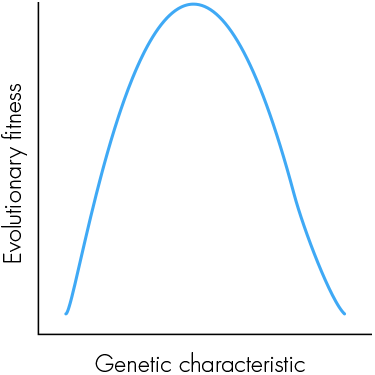
The graph below is the basis of an insight originally articulated by the eminent statistician and evolutionist Sir Ronald Fisher. Imagine that you as an individual are situated at some point on the curve. Presumably this would be at some point near the top, since the fact that you exist implies that you are a product of evolutionarily fit ancestors. If you have a large genetic mutation, you are likely to move to a different point on the curve, which will probably be bad for you. Yet, Fisher asserted, if the mutation were small enough, it would have a 50 percent chance of being good for you. Can you figure out why this should be so?

What will happen if we rotate the graph into a three-dimensional figure looking like a rounded cone and use it to represent not one but thousands of different characteristics? In what way will this modify these conclusions?

I can do no better than to quote the answer given by Daniel McLaury:

In fact, we need almost no assumption as to the nature of the curve, so long as we can assume it’s smooth. Provided we are not exactly at a local maximum of fitness (which, given a unimodal fitness function like the one shown, is actual “maximum fitness”), then fitness is either increasing or decreasing with respect to the characteristic in question. In the former case, a small move to the left (i.e., small enough not to leap right over a local maximum) will hurt, and a small move to the right will help. In the latter case, the situation is reversed. In either case, provided there’s a 50-50 chance to move left or right then there’s a 50/50 chance that the change will be a positive one.

The situation is not changed in higher dimensions, as all change happens in some direction. We may simply restrict our attention to the direction the change occurs in, reducing to the one-dimensional case considered before.

There has been some debate in the comments section regarding an answer given by Michael, who treated the multidimensional figure purely mathematically and came up with an answer of less than 50 percent for a small, but not infinitesimal, change. This is, however, a “trick question.” Our third dimension is created by juxtaposing hundreds of different traits with their own upside-down U profiles of fitness. Each individual line making up this 3-D figure is discrete and represents a different trait that may have no interaction with the one adjacent to it. In effect, we are adding a discrete categorical axis, not a continuous numerical one. So it is not kosher to perform the kinds of mathematical operations that Michael did to make his argument. This is the argument that I believe Hans makes. The mathematics of evolutionary fitness is extremely interesting and has shown that there is a great deal of evolutionary change that is neutral with respect to fitness. Perhaps we can go into it in more depth in a future column.

The Quanta T-shirt for this month goes to Daniel McLaury for his interesting comments on both questions.

See you soon for new insights.