How Geometry, Data and Neighbors Predict Your Favorite Movies

BIG MOUTH for Quanta Magazine
Introduction
Adrienne is a Marvel movie fanatic: Her favorite films all involve the Hulk, Thor or Black Panther. Brandon prefers animated features like Inside Out, The Incredibles and anything with Buzz Lightyear. I like both kinds, although I’m probably closer to Adrienne than Brandon. And I might skew a little toward Cora, who loves thrillers like Get Out and The Shining.
Whose movie preferences are closest to yours: Adrienne’s, Brandon’s or Cora’s? And how far are your cinematic tastes from those of the other two? It might seem strange to ask “how far” here. That’s a question about distance, after all. What does distance mean when it comes to which movies you like? How would we measure it?
As strange as it may seem, companies like Netflix measure and make use of these kinds of distances every day. By watching what you watch and analyzing the data, they create measurements of your fondness for comedies, romances, documentaries and other kinds of movies, and use that information to imagine your position in the abstract space of movie preferences. Then, by identifying the people closest to you in this abstract space — your nearest neighbors, so to speak — Netflix can recommend new things for you to watch: namely, the things your neighbors like.
When it comes to these kinds of predictive engines, knowing who is closest to whom is crucial in understanding, classifying and analyzing complex data sets. And it all starts with some simple ideas developed in high school geometry.
Let’s start by thinking of Adrienne and Brandon as points in the plane.

In reality, movie preference space is much bigger and more complex (and real recommendation engines are much more sophisticated) than what we are imagining here, but this is a friendly place from which to start exploring the math.
To help see if we’re closer to A or B, let’s draw a perpendicular bisector — a line segment that is perpendicular to $latex \overline{AB} $ and cuts it in half. The perpendicular bisector is a very useful tool in Euclidean geometry. Anytime you need to cut something in half, there are perpendicular bisectors around.
In the plane, the perpendicular bisector of a line segment is a line, as seen below.
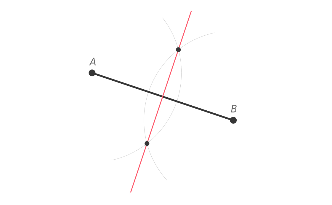
A typical construction of line segment $latex \overline{AB} $’s perpendicular bisector, using intersecting congruent circles centered at A and B.
One important property of perpendicular bisectors is that its points are equidistant from the endpoints of the segment it bisects. This intimately connects perpendicular bisectors to isosceles triangles — triangles with two sides of the same length. Suppose a point Q lies on the perpendicular bisector of segment $latex \overline{AB} $, like this.
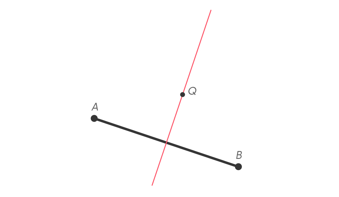
Because it lies on the perpendicular bisector of segment $latex \overline{AB} $, point Q is equidistant to A and B. That is, QA = QB. If Q represents Quentin, then Quentin is just as close to Adrienne as to Brandon.
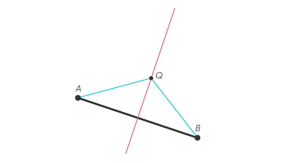
We can prove QA = QB using basic properties of either triangles or reflections, but we can also demonstrate it by folding. If you draw this diagram on a sheet of paper and fold along the perpendicular bisector, you’ll see A line up with B. And since Q lies on the crease, the segment $latex \overline{QA} $ will overlap with $latex \overline{QB} $ . This means they must be the same length. This makes $latex \Delta AQB $ an isosceles triangle. In fact, the perpendicular bisector of $latex \overline{AB} $ is the set of all the points that make an isosceles triangle with $latex \overline{AB} $ as its base. (There is one situation we should be slightly worried about. Can you spot it?)
Since every point on the perpendicular bisector of segment $latex \overline{AB} $ is equidistant to A and B, we have another powerful way to think about the perpendicular bisector: as a dividing line.
Let’s put Yvette in our plane, at some point Y that is not on the perpendicular bisector of $latex \overline{AB} $.
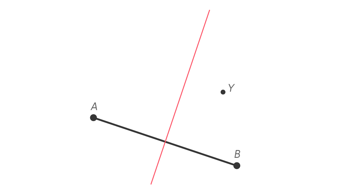
We know immediately that Y is not equidistant to A and B, but we can say more. We can geometrically show that Yvette is closer to Brandon than to Adrienne. Imagine segments $latex \overline{YA} $ and $latex \overline{YB} $.
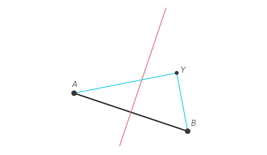
We can show that YB < YA by adding a little something to our diagram. Let I be the intersection of $latex \overline{YA} $ and the perpendicular bisector, and draw a new segment $latex \overline{IB} $.
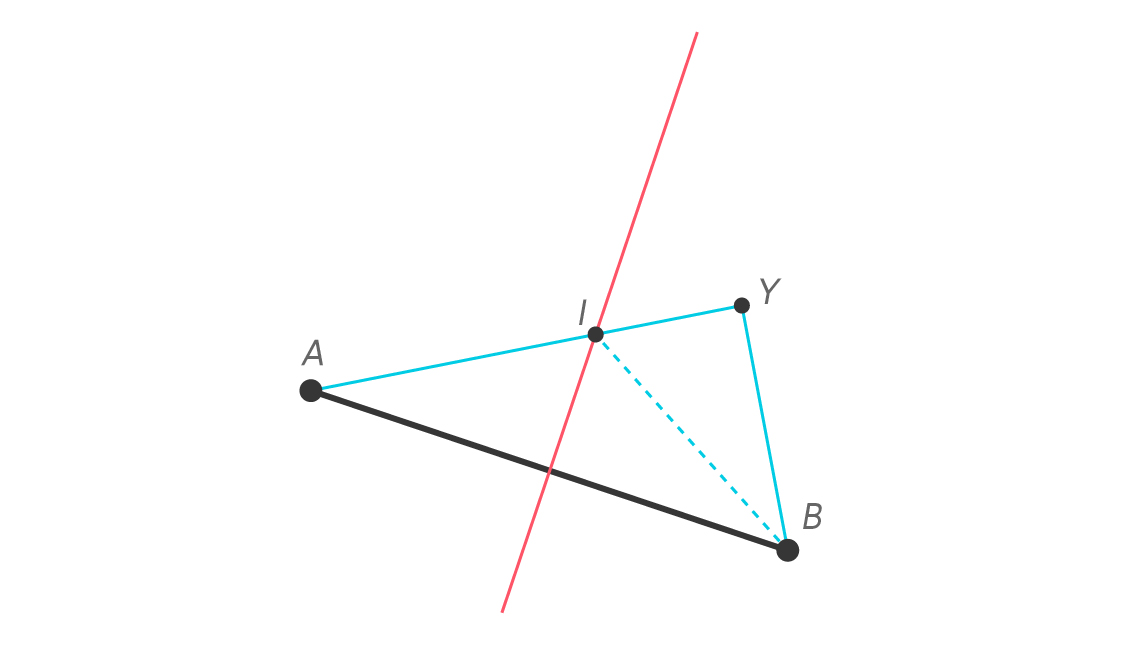
Since I is on the perpendicular bisector of $latex \overline{AB} $, we know I is equidistant to A and B. This means IA = IB. Using some basic facts about line segments, we see that
YA = YI + IA = YI + IB
But in a triangle, any one side must be shorter than the other two sides put together. This fundamental fact, called the “triangle inequality,” basically says the shortest path between two points is the straight line segment that connects them. Applying the triangle inequality in $latex \Delta YIB $ gives us
YB < YI + IB
And since YI + IA = YI + IB = YA, we see that YB < YA.
Notice that Yvette is on Brandon’s side of $latex \overline{AB} $’s perpendicular bisector. That tells us that Yvette is closer to Brandon than to Adrienne. Similarly, everything on Adrienne’s side of $latex \overline{AB} $’s perpendicular bisector is closer to Adrienne than to Brandon. So the perpendicular bisector of $latex \overline{AB} $ divides the plane into two sets: things that are closer to A and things that are closer to B. If you want to know whom you are closer to, you just need to know which side of the perpendicular bisector you are on.
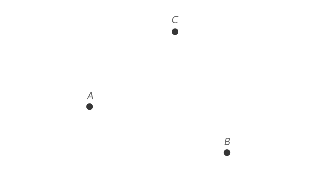
This strategy works with more than two points. Let’s add Cora.
Here’s the perpendicular bisector of $latex \overline{AB} $.
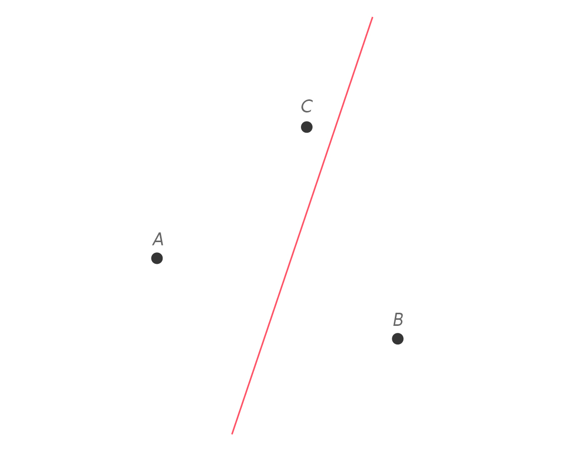
We know this divides the plane into two regions: things that are closer to A, and things that are closer to B. Notice that since C lies on A’s side, C is closer to A than B. Now let’s construct the perpendicular bisector of line segment $latex \overline{AC} $.
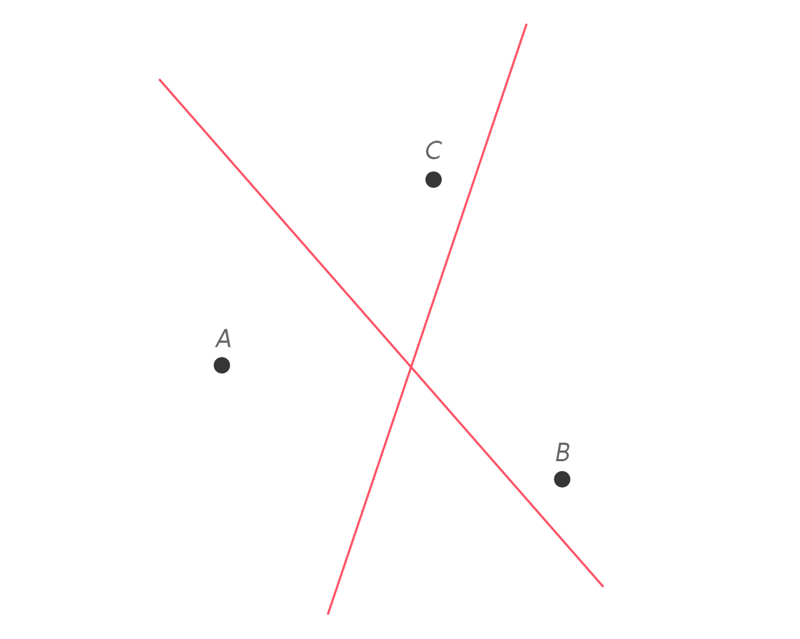
This also divides the plane into two regions: things that are closer to A and things that are closer to C. Notice that B is closer to C than to A, since it lies on the C side of $latex \overline{AC} $’s perpendicular bisector.
Several remarkable things happen when we construct the remaining perpendicular bisector of $latex \overline{BC} $.
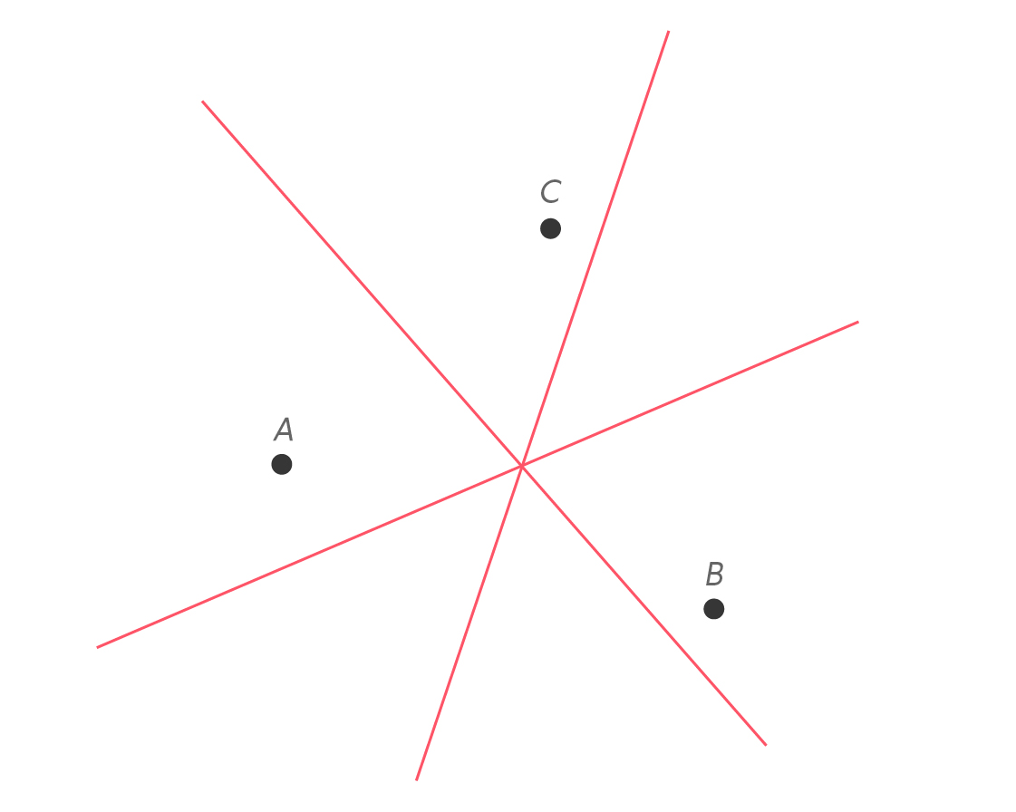
First, all three perpendicular bisectors intersect at a single point. This “concurrency” of the perpendicular bisectors of $latex \overline{AB} $, $latex \overline{BC} $ and $latex \overline{AC} $ is almost magical and is one of the loveliest results in elementary geometry. And it’s not hard to see why it happens. Let’s go back to when we had just the two perpendicular bisectors.
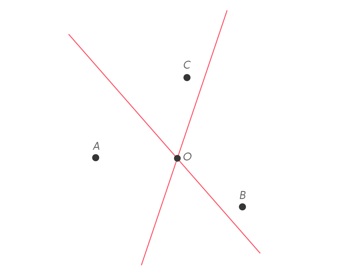
Let’s call the intersection of these two perpendicular bisectors point O. Because it’s the point of intersection, O lies on both perpendicular bisectors. Since it’s on the perpendicular bisector of $latex \overline{AB} $, we know that OA = OB . But O also lies on the perpendicular bisector of $latex \overline{AC} $, which means OA = OC.
But if OA = OB and OA = OC, then OB = OC. This means O must lie on the perpendicular bisector of $latex \overline{BC} $, and all three perpendicular bisectors pass through a single point!
This remarkable concurrency isn’t the only remarkable thing happening here. Let’s take a look at the regions created by these three intersecting lines.
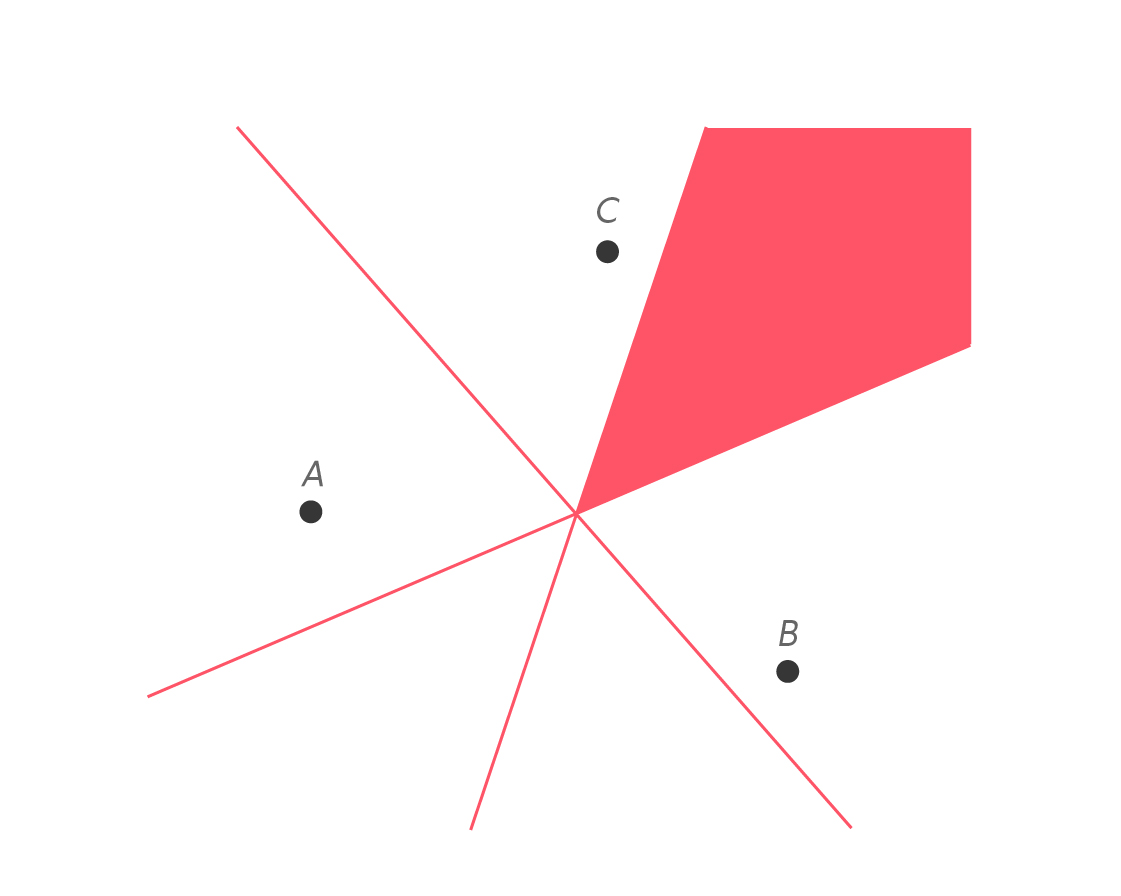
Consider the region in red. These points are on the C side of the perpendicular bisector of $latex \overline{BC} $, so they are closer to C than to B. But they are also on the C side of the perpendicular bisector of $latex \overline{AC} $, which means they are closer to C than to A. Thus, every point in this region is closer to C than to either A or B.
Similar reasoning allows us to fill in the rest of the diagram like this.
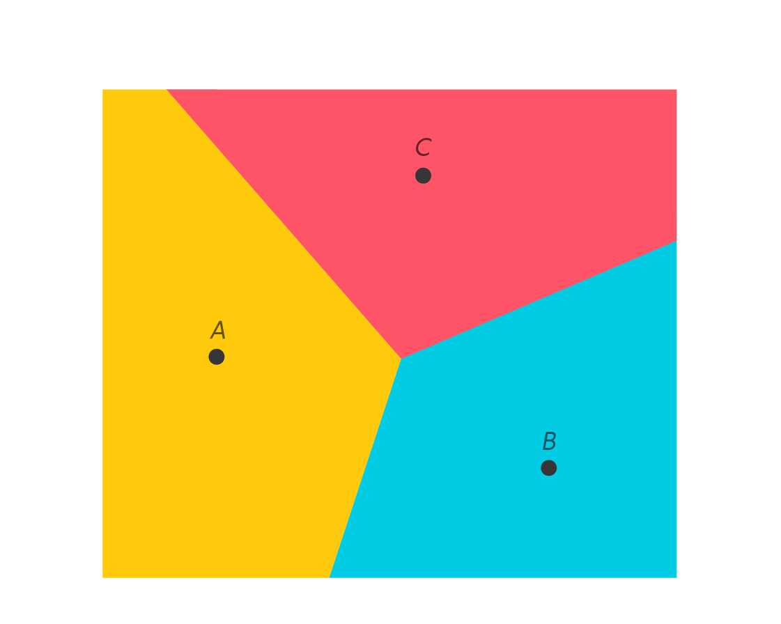
Clearly, the red points are all those closest to C, the yellow points are those closest to A, and the blue points are those closest to B. Using perpendicular bisectors, we have created a “Voronoi diagram”: a partitioning of the plane into regions of points that have the same “nearest neighbor” among the points A, B and C.
In this simplistic imagining of movie preference space, here I am at point P: closer to Adrienne’s superheroes than Brandon’s toy stories, but heading toward Cora and her horror shows.

Since I’m in the yellow region, this partition tells me that Adrienne is my nearest neighbor: If I’m looking for a new movie to enjoy, trying out something she likes would be a good bet. And, in a movie preference space with millions of viewers, there will be even nearer neighbors whose preferences will better match mine than Adrienne’s will. As you watch movies and get located in this space, your nearest neighbor can recommend movies for you, too.
This geometric analysis works for any number of points in any number of dimensions. The only thing that really changes is the nature of perpendicular bisector itself. In the plane, a perpendicular bisector is a line, but in three-dimensional space, a perpendicular bisector is a plane. And in 10-dimensional space, a perpendicular bisector is whatever splits 10-dimensional space in half (a nine-dimensional hyperplane).
While the approach may stay the same, computations become more difficult as the dataset gets more complex. Having more dimensions means more coordinates for each data point, which means more complicated distance calculations. And since you have to find the perpendicular bisector for each pair of points, the number you must find grows very quickly as the number of points increases: With three points, there are three perpendicular bisectors, but with 100 points, there are nearly 5,000.
In a space of millions of points with thousands of coordinates each, computing all the necessary distances can become computationally infeasible. To deal with this complexity, mathematicians and computer scientists have developed algorithms to partition space and find nearest neighbors that are much more efficient than simply finding all the perpendicular bisectors. This often involves estimating nearest neighbors rather than locating them exactly, making the classic trade in mathematics of accuracy for simplicity.
Things get even more complicated when we start using different notions of distance. We’ve been using the standard “Euclidean” definition of distance, the one that relies on straight lines and the Pythagorean theorem. But different datasets require different measures of distance, and different measures of distance give rise to different, and more complex, partitions of space.
For example, here’s what a Voronoi diagram can look like using what’s known as “taxicab distance.”

In a world measured by “taxicab distance,” the shortest path between two points isn’t the one the crow flies; it’s the one the taxi drives, where only horizontal and vertical streets are available. This notion of distance can be useful in real-life applications like urban planning — deciding how hospitals should be spaced out depends more on driving distance than on flying distance.
“Taxicab distance” also shows up in abstract contexts, as do other kinds of distance, like “edit distance” (a measure of how different two strings of words or symbols are) and graph distance (the length of the shortest path between two nodes of a graph). The ability to model distance in different ways in different spaces is a source of great mathematical power, but it also has the potential to make each kind of partitioning problem complicated in its own unique way.
This is partly why mathematicians were so excited and surprised by the recent discovery of a general-purpose method for finding nearest neighbors in complex data sets. It even surprised the researchers who discovered it: They originally set out to prove that it was impossible.
In a high-dimensional movie preference space, researchers can create multiple notions of distance. They might look at differences in how users rate movies, how long they watch them, what previews they click on, and more. The data are endless and can be combined in endless ways. The same is true of modeling patients in the space of health statistics, where predictive engines make educated guesses about what illness might afflict you next, and of how match-making services pair up users who are just the right distance apart in relationship space (close, but probably not too close).
But even across these vastly different spaces, there are general techniques for finding nearest neighbors. And whether it’s measured in movie preferences, medical symptoms or relationship qualities, the distances to our nearest neighbors can tell us a lot about ourselves.
Exercises
- Above, the perpendicular bisector of $latex \overline{AB} $ was described as “the set of all points that make an isosceles triangle with $latex \overline{AB} $ as its base,” but it was noted that there was one situation that we should be slightly worried about. What situation is that?
- Any two distinct points have a unique perpendicular bisector. What is the maximum number of perpendicular bisectors found among 100 distinct points? Could it be possible to have fewer than this maximum number?
- In the Cartesian plane, how many lattice points (points with integer coefficients) are exactly 10 units away from the origin, using the “taxicab” distance?
- The perpendicular bisector of $latex \overline{AB} $ is the set of all points equidistant from A and B. In the plane, this makes a line. What does the set of all points twice as far from A as from B make in the plane?
Answers
Click for Answer 1: The midpoint of $latex \overline{AB} $ is on the perpendicular bisector, but it doesn’t really make a triangle with $latex \overline{AB} $ as its base, as the points are collinear. Or maybe it makes a degenerate triangle!
Click for Answer 2: This is equal to the number of pairs of points among 100 total points, which is $latex _{100}C_2 $ = $latex \begin{pmatrix} 100 \\ 2 \end{pmatrix} $ = $latex \frac{100!}{98!2!} $ = $latex \frac{100⋅99}{2}$ = 4,950. And yes, some perpendicular bisectors could overlap, if two different pairs of points were collinear and shared the same midpoint.
Click for Answer 3: The points are (10,0), (9,1), (8,2), …, (1,9), then (0,10), (-1,9), …, (-9,1), then (-10,0), …, (-1, -9), then (0,-10), …, (9, -1). Four sets of 10 points, so 40 points.
Click for Answer 4: A circle. Proof is left to the reader.
Corrected on May 22, 2019: Due to a typographical error, an earlier version of this column gave the incorrect reason for point B being closer to point C in one of the diagrams. Also, because of a change in the color scheme of a different diagram, the column previously referred incorrectly to "green" points that actually appeared as blue points. Both errors have been corrected.


